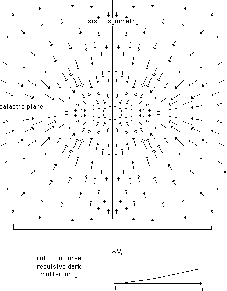
...Now we add the galaxy, which reinforces the gravitational field, mainly close to the center, where the pressure force balances the field. As shown on figure 3 the gravitational force has a confining z-component. Such a phenomenon might explain the anomalous large z-velocities, evidenced by Bahcall ([4] and [5]) for K stars. A complete and systematic study should be carried out by this method. Finding these large velocities, Bahcall concludes that some dark matter must be present in the disk of the galaxies. According to our model, that could be due to the repulsive effect of the surrounding repulsive dark matter : an alternative interpretation.

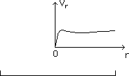
...In general, starting from observational data, people can compute the distribution rdm(r,z) of "conventional" dark matter in space. Similarly, from the same observational data, it is possible to build a corresponding distribution r*(r,z) of repulsive repulsive dark matter, through the method presented above. The local intensity of the gravitational field depends on the chosen distribution. Here we have used a system of concentric shells figured as a set of thick ellipsoids with the same excentricies, but the excentricities might be different. Any kind of distribution r*(r,z) of repulsive repulsive dark matter can be managed by this method. We get a rotation curve, corresponding to gas orbiting in the z = 0 plane, good-looking, as shown on figure 4. The scale, shown, corresponds to figure 1.

 
...The repulsive dark matter environment acts as a "box". The flatter that box, the stronger the corresponding impact on the z-confinment effect is. With the chosen parameters, the z-confinment enlarges the velocity of the stars located at z = 0.2 dg (where dg is the overall diameter of the galaxy) by a factor 1.4.

...The global gravitational field (acting on the repulsive dark matter) tends to enlarge the hole. But its pressure gradient balances it : if the galaxy was removed, the repulsive dark matter would fill the hole. The repulsive dark matter distribution was shaped on empirical grounds, through numerous trials and various sets of massive ellipsoids. It could be a starting point for full 3d numerical simulations, which are beyond our todays’ computational possibilities.
 

3) Geometrical framework. Field equations.

...As previously stated, repulsive darkmatter acts if its mass were negative. If this type of matter were actually present in ou universe, problems would arise in consesquence of the corresponding particles’ negative energies. This difficulty can be avoided endowing the universe with a new geometrical structure.

...As presented in former papers ([6] and [7]) we assume that the geometry of the Universe corresponds to the two-fold cover of a four dimensional manifold M4. We call these adjacent folds F and F*. M4 is a set of points. We can describe these points in an arbitrary system of coordinates {z i}. M and M* being the corresponding points of the folds F and F*, they are described by the same set of coordinates and then linked by this involutive mapping. The manifold M4 can be considered as a "skeleton manifold", as we use it to build the involutive mapping linking M and M*. We shall say these points are adjacent. We introduce two metrics g and g* and assume they describe the geometries of the two folds. We assume they are both Riemanian, with common signature (+ - - -). The physics in the two folds are identical, and Special Relativity holds each of them. We assume that light follows null-geodesics in each folds, but, on geometrical grounds, light cannot travel from a fold to the other one.

The set of coupled field equations ruling the system is a free choice. Let us take :

(3)

(4)

S and S* are two geometric tensors built from the two Riemanian metrics g and g* . The second members they are sums of tensors describing the content of energy-matter. The subscript r refers to radiation (and "dark radiation") and the subscript m to matter (and repulsive dark matter).

Tr : contribution of "normal photons" j , travelling in fold F. Tends to produce a positive curvature in folds F and F*.

T*r : contribution of "dark photons" j* , travelling in fold F*. Tends to create a positive curvature in folds F and F*.

Tm : contribution of "normal matter", travelling in fold F. Tends to create a positive curvature in that fold and a negative curvature in fold F* (due to the minus sign in (3).

T*m : contribution of "repulsive dark matter", travelling in fold F*.Tends to create a positive curvature in that fold and a negative curvature in fold F (due to the minus sign in (4).
 

The system (3) + (4) means :

- When "normal photons" j are converted into matter and antimatter, it does not change their (positive) contribution to the curvature, in the fold F. But this contribution becomes negative for the fold F* .

- When "dark photons" j* are converted into repulsive dark matter and anti repulsive dark matter, this does not change their (positive) contribution to the curvature of the fold F*, but this contribution becomes negative in the fold F.

- When a particle-antiparticle pair is converted into photons j , in the fold F, their contribution becomes positive for both folds.

- When a dark particule-anti dark particle pair is converted into dark photons j*, their contribution becomes positive for both folds.

At this stage this sign flip is the weak point of the model. Another description of the radiative era will be given in the next paper, where this difficulty is avoided.

...In classical general relativy the local scalar curvature can be positive or null. In such a model the scalar curvature can be locally negative. When the curvature is negative, in a fold, it is an "induced curvature", due to the presence of matter in the adjacent portion of the other fold. If R is the local scalar cuvature in the fold F and R* the one in the fold F*, we simply have R* = - R .

Assuming the two universes to be isotropic and homogeneous, the metrics, in spherical coordinates, are :

(5)

(6)

where (u , q , j) are common space-markers and { k , k* } curvature indixes. We take same light velocity c and cosmic time t in the folds.

As in the standard model, we find two stages. During the first one, the radiation dominates, and the equations reduce to :

(7)

During this radiative era we assume R = R* , r = r * , p = p* . The solution fits the standard model, and for a null curvature index we get :

 
(8)

...In the second stage, when the two universes get cooled enough (we assume that the decoupling occurs at the same time in both folds, but this could be different and would require another study), matter dominates in both folds and the system becomes :

(9)

(10)

 
We get the following system of four differential equations :

(11-a)

(11- b)

(11- c)

(11- d)