15) The radiative era..

The idea is that the so-called
constants of physics behave like absolute constants during the matter era, but
change drastically during the radiative era. It may look very artificial, but
this idea may solve the problem of the homogeneity of the early universe, as
recently pointed out by several authors, like Magueijo (1999), but was
discovered by the author 13 years before, at the end of the eighties ([44],[45], [46] ) and developed later ( [4] and[47] ). First,
notice that the choice of the time marker t remains arbitrary. It is nothing
but “the way we think the things happened”. Absolute time has no meaning in
cosmology. Any phenomenon does not “exist” if there is no observer in the
Universe to look at it, to compare a succession of events to his proper time
flow. At present time all is compared to the time of the observer, the way he
lives. But past and future depends on the way he imagines it, for he cannot travel in past or future. Past and
future are nothing but images we shape. We will say that these images are
correct if they fit peculiar local phenomena, that we call “observations”,
“measurements”. Consider the “constants of physics”. They were discovered quite
recently. They are the light speed c , the gravitational constant G, the Planck
constant h , the masses of particles, the unit
electric charge e, the permittivity of vacuum eo , and some others. Measurements performed in
labs show no significant change. People have tried to study the impact over
large period of time of a change of these constants on various cosmic
phenomena. But they moved these constants one after the other, independently.
In such conditions one can show that any light variation of an isolated
constant produces contradictions with observational data. But what about joint
variations ? Surprinsingly we may conceive a joint variation of all the
constant, which cannot be evidenced in lab, for the lab’s instruments are built
with the basic equations of physics. If this gauge process keeps these
equations invariant, it will be impossible to evidence the variation of any
constant, for the instruments and the constants they are supposed to measure
experience parallel drifts. Imagine you want to measure the length of an iron
table, with an iron scaled rule. Both are at room temperature. If the table’s
length is found constant in time, you cannot sware this length does not vary,
for this table and your scaled rule may experience a room temperature variation
and expand in the same way. Let us
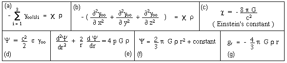
search such basic gauge process. Consider for example the field equation, where
we find the Einstein constant. We assume the divergence of this equation is
zero which, in Newtonian approximation, corresponds to the conservation of
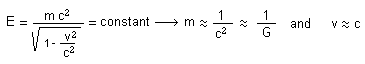
matter and energy. If it is not, we must deal with source term. According to
this hypothesis the Einstein constant c must be an absolute constant. Does it imply that G and c must be
absolute constants ? Definitively not. It only implies that :
![]()
As
introduced first in 1988 we assume that the energies, all kind of energies, are
conserved, but not the masses, electric
charge and so on. This gives, for example :
In
physics all students know the technique called dimensional analysis. Given a
physical problem, ruled by an equation, or a set of equations, we produce
characteristic lengths, times and numbers, composed with constants and
laboratory condition data. Now we consider that all what is present in the
equation may vary, including the “constants”. We put everything into a
non-dimensional form. Consider for example the Boltzmann equation :
![]()
We
introduce a characteristic length scale R and a characteristic time scale T :

The
equation becomes
:
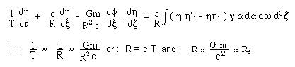
We
see that the Schwarzschild length varies like the scale factor R. To sum up
get :

We see that the Jeans length Lj varies like R, while Jeans time tj varies like T. R and T are linked through a relation which evokes a Friedman model. But if one looks that closer and see it as a gauge relation, it means that the Kepler laws are also invariant :
![]()
By the way, introducing pressures (as energy
densities) we get the gauge variations of
these parameters and see that the subsequent energies are conserved (in
this model all kinds of energy are conserved during the radiative era). We have
figured the way the speed of light c varies with the energy density when
radiation dominates.
![]()
Now
consider the Schrödinger equation :
![]()
Introduce
non-dimensional potential expression and transform this equation :
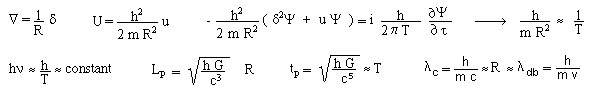
As a result, the energy is unchanged by this gauge process. The Planck constant h grows with T, as conjectured first by Milne [48]. The characteristic lengths :
vary like the space scale factor
R, while the Planck time tp varies like the time scale factor T.
From this point of view, the evolution, during the radiative era is conceived
as a gauge process. This makes the “Planck barrier” questionable. Does the
“pre-quantic” epoch has a real meaning ? Now, to finish the job we have to deal
with Maxwell equations.
Continue
to perform that sort of “generalized dimensional analysis”. We get :
In
order to maintain the structure of the atoms during the evolution process we
assume the fine structure constant is an absolute constant, which gives the
whole solution :
![]()
We
get easily :
As we can see, during the radiative era, is the cosmic evolution is identified to a gauge process, all characteristic lengths vary like R (above, the Bohr radius), all the characteristic times vary like T, all the energies are constant.
![]()
![]()
All the constants,
space and time scales are involved in this gauge process, which can be
described chosing any of them. We can take T as our time-marker t .
Next,
the variation of the constants, during the radiative era, versus the radiative
pressure pr :
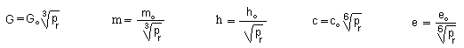
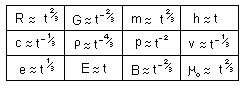
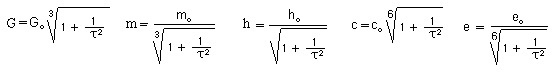
If
we assume that the values of the constants depend on the radiative pressure,
introducing a critical value pcr, to be defined, we can write :
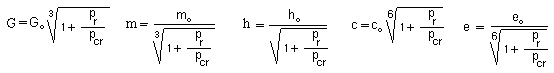
Go , mo , ho , co , eo correspond to the today’s values. We assume that this critical conditions are achieved for a value t = tcr of the chosen time-marker.
![]()
which
corresponds to figure 16.
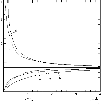
Fig. 16 : Variation
of the constants during the radiative era.
t >> tcr corresponds
to matter era
16) The homogeneity of the Universe.
Any
model requires an observational confirmation. Figure 17, left, the classical
paradox of the homogeneity of the early Universe. “Classical explanation” : the
“Inflation Theory”, requiring heavy hypothesis. Today, some people begins to
think about a variable constants model, including a secular variation of c. The
called it “VLS” : “variable light speed”. In fact I developed this idea in 1988
[44]. With the suggested time-variation of c ,
which with the precedent section the horizon varies like R(t) which ensures
homogeneity at any time.
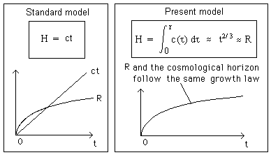
Fig. 17 : The
horizon, according to the standard model and to the present model.
17) When the adverb “before” fails.
As
said above, a time marker corresponds to an arbitrary choice. It has no
intrinsic meaning. In the standard model if we deal with the distant past of
the Universe, the temperature rises and elements’ velocities tend to c. All
particles become relativistic, so that a question arises : “how to build a
clock, with which material ?”. When we look at a clock, what do we look at ? To
the rotation of a needle. A turn corresponds to a minute, or hour. A turn of the
Earth around the Sun corresponds to a year. Whatever we call it, this 360°
rotation has a physically real meaning. It is an undeniable event. Similarly we
can consider a reference system composed by two masses m orbiting around their
common centre of gravity. We may call it our “elementary clock”. In a gas at
thermodynamic equilibrium the available energy is distributed in translational energy, the rotational energy,
vibrational energy. A couple of particles orbiting around their common centre
of gravity is conceivable if the energy of the system is comparable to the
energy of free particles, which cruise around. In a variable constant system
this is possible. Then we can count the number of turns, using the time-marker
t, which has no real significance : it’s only a chronological marker.
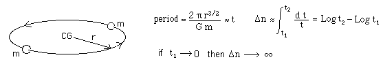
Fig.18 : The
elementary clock.
What does it mean ?
According to this description of the Universe, an infinite number of
“elementary events” occurred in the past. If this clock corresponds to a
measure of time, past is infinite and the time-marker t is nothing but a
fiction. Let’s give an image. Suppose you visit an editor and say “I want to
publish a two inches thick book”. Depends on the width of the pages. You may
deceive the editor if you use pages whose width tends to zero when trying to
read “the first pages”. Although the global width of the book seemed finite it
tells a infinite story. The good question the editor must ak you is “how many
types in your book, how many sentences, words, letters ?”. A letter of your
book can be compared to an “elementary event”. As your book, called “Universe
story”, going towards the past, shows an infinite number of “elementary
events”, it has… no beginning and you will never succeed in reading the
foreword of the author. By the way, as shown in reference [4] the
number of turns of our elementary clock identifies to the entropy per baryon.
Log t is also called “conformal time”. In effect if chosen as a new time-marker
the metric becomes conformally flat :
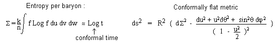
In
the precedent section we found that the Planck time vary like the time-marker
t. It means that when one goes back to the so-called “initial singularity (t =
0)” the Planck time shrinks. What does it mean ? I haven’t the answer. Anyway
this model doesn’t clear up all problems. We don’t deal with strong and weak
interaction. It’s only a different glimpse on what we call “time”.
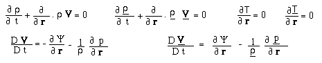
17) Joint gravitational instabilities.
In section 3 we have presented a model of a galaxy confined by its repulsive twin matter environment. This work was semi-empirical. In the present section we present a spherically symmetric exact solution. If we start from the coupled field equation, we assume that it is divergenceless
![]()
From such
equations one can derive Euler equation. The method is completely similar to
the one applying to the Einstein equation.
Coupled
to Poisson equation :
![]()
The
classical perturbation method gives two Jeans like coupled equations, Lj and Lj
being characteristic Jeans lengths.
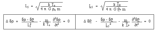
A steady-state spherically symmetric solution, with initial conditions :
![]()
![]()
On
figure 19 the typical numerical solution.
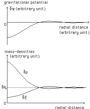
Fig.
19 : Joint gravitational instabilities. Formation of a clump of matter
surrounded by repulsive twin matter environment.
The general feature of the curves depends on the initial conditions. The chosen conditions are arbitrary and correspond to the equal mass densities and equal thermal velocities in the two folds. Anyway, we find an interesting feature. On figure 19 bis we can plot the gravitational field direction :
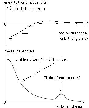
Fig 19 bis : "Dark matter halo" effect
The gravitational field induces a gravitational lensing effect. This last is a measure of the gravitational field, whatever is the source of this field. In our theory, the ordinary matter, the one of ou "fold", brings its own contribution. The "twin matter" bring its contribution too ( it behaves like negative mass material ).
If we choose to consider that the observed strong lensing effects are due to some mysterious "dark matter", given the gravitational fiel and the distribution of visible matter one can compute the distribution of this dark matter, if it does exist. On figure 19bis we observe an inversion of the direction of the gravitational field, which goes with a corresponding variation of the local gravitational lensing. Following the model of the matter plus dark matter we could compute the distribution of dark matter which would give the corresponding lensing effects. Considering the figure at the top of Fig 19 bis we would deduce that this cluster is surrounded by "an hollow shell of dark matter". The picture at the bottom evokes such conclusion.
As we know, the space Hubble telescope has recently discovered a "halo f dark matter". See the next figure.
Fig 19 ter : The "halo of dark matter" discovered by the Hubble space telescope in 2007, may. As "deduced from computation".
Surprinzingly this halo is centered on the visible galactic cluster. We think that it does not correspond to a plane structure but to a spherically symmetric structure. We predict that similar structures should be discovered soon. In all cases the "halo" will be centered of the cluster, so that the astrophysicist will admit this is not a halo but "some sort of hollow structure.
The halo structure could be considered as the result of an old encounter ( looking "like a smoke ring" ).
Suppose my prediction would be confirmed. If astrophysicists have to admit that these observations correspond to spherically symmetric structure, how will they modelize this hollow dark matter shell ?
If it is confirmed, this could bring the elements to make a choice between the matter plus dark matter model and the twin universe model.
18)
The confinement of spheroidal galaxies.
In section 7, figure 11, we said that the field due to a hole in a uniform negative energy matter was equivalent to the field created by an equivalent sphere, filled by positive energy matter and surrounded by void. It has now to be justified. Let us recall how the link to Poisson equation is built in classical theory ( see for example[52] ).
![]()
This gives (a) :
The one writes (b). With (d) and (c) the equation (b) is identified to Poisson equation. But notice immediately that the given perturbed metric corresponds to steady-state conditions. This is conceivable only if the zero order solution (the Lorentz metric) corresponds to an empty universe, where no gravitational force and no pressure are acting.
![]()
Then there is a link
between the field and the Poisson equations. But is the Universe is supposed to
be non-empty and uniform this method does not hold any longer, for we cannot
refer to steady state metric. What is the impact ? We cannot define a
gravitational potential in an uniform universe, filled by constant density
material. If we look at the Poisson equation (e), written in spherical
coordinates and if we suppose r is a constant, we find the spherically solution (f) and the
corresponding gravity field is (g). Isn’t surprinzing to find a non-zero
gravitational force, pointing towards an arbitrary centre of coordinates and
tending to infinite with radial distance ? Explanation : this pseudo-solution
is not correct, for Poisson equation does not exist in an steady state uniform
universe. The field is zero everywhere, which looks more physical.
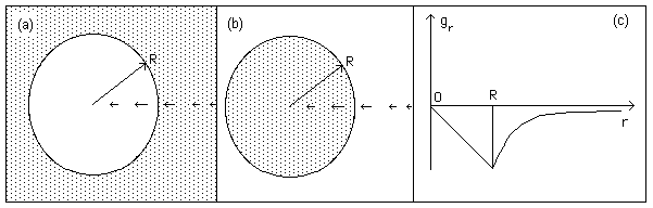
Fig. 20 :
Spherical hole in a constant density twin matter distribution
and associated gravitational potential.
The
figure (b) shows the gravitational field around and inside a sphere filled
by constant positive density material (like the Earth). In (c) the associated
gravitational potential. If we reverse the arrows of (b) we get the field
associated to a sphere filled by negative mass. If this is added to (a) we
get an uniform and unbounded region, filled by negative mass, with a zero
field, so that (a) figure the field inside a spherical cavity, which is non-zero.
We get a confining effect and the intensity of the field is maximum at the
internal border. This explains why the spiral galaxies keeps their arms and
why the decrease of the gas density of the disk is so abrupt at periphery.
Paper's Summary